Understanding Flare Rates of Young Stars with Machine Learning

Adina Feinstein, Ben Montet, Megan Ansdell, Brian Nord, Jacob Bean, Max Gunther, Michael Gully-Santiago, & Josh Schlieder

arXiv:2005.07710

TL;DR

M dwarfs have consistently high flare rates across the first 800 Myr, while hotter stars have fewer flares over time.

M dwarfs with T_eff < 3200 K have the highest normalized energy flares in the sample.

High flare rates seen on young stars cause exoplanet atmospheres too lose 4-7% more atmospheric mass.

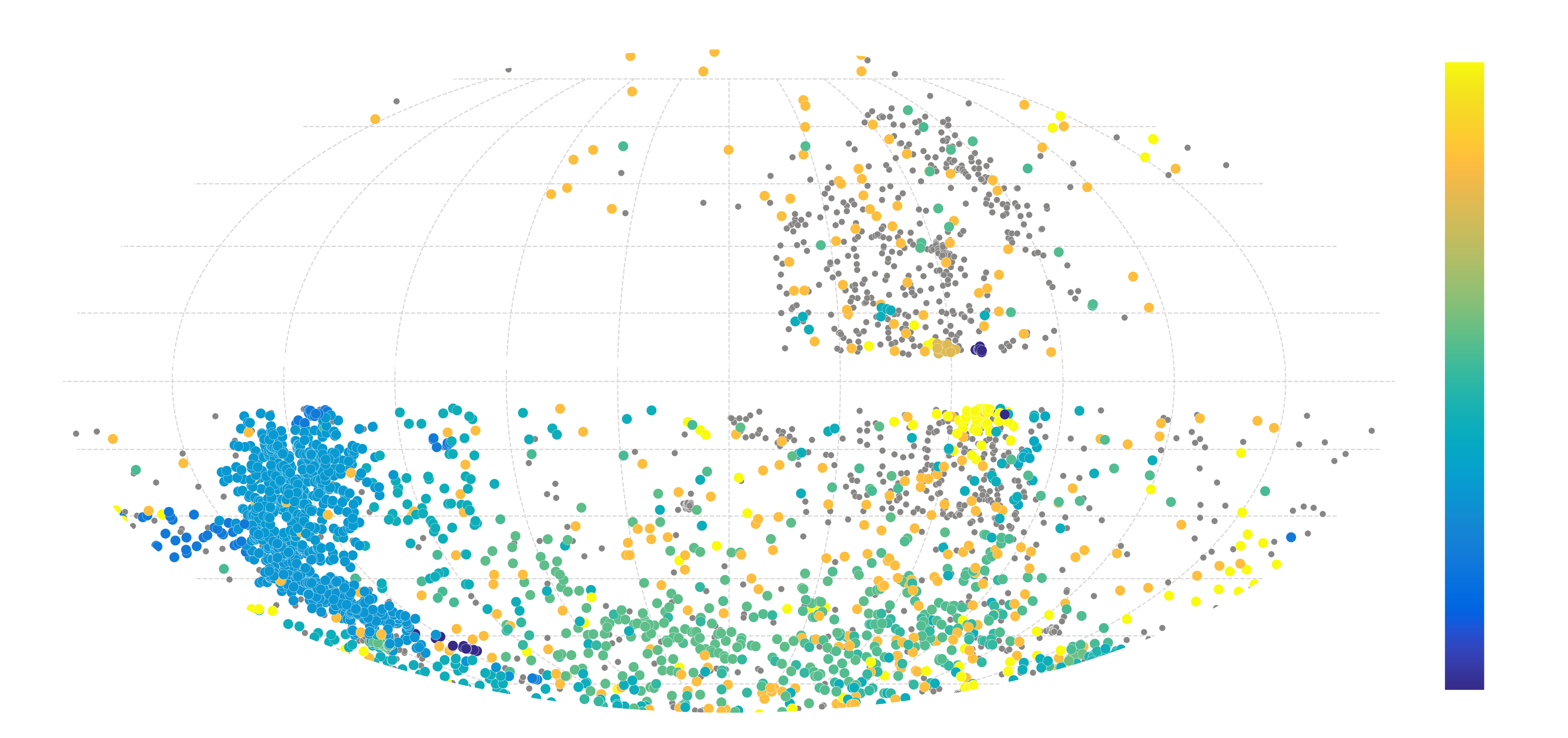
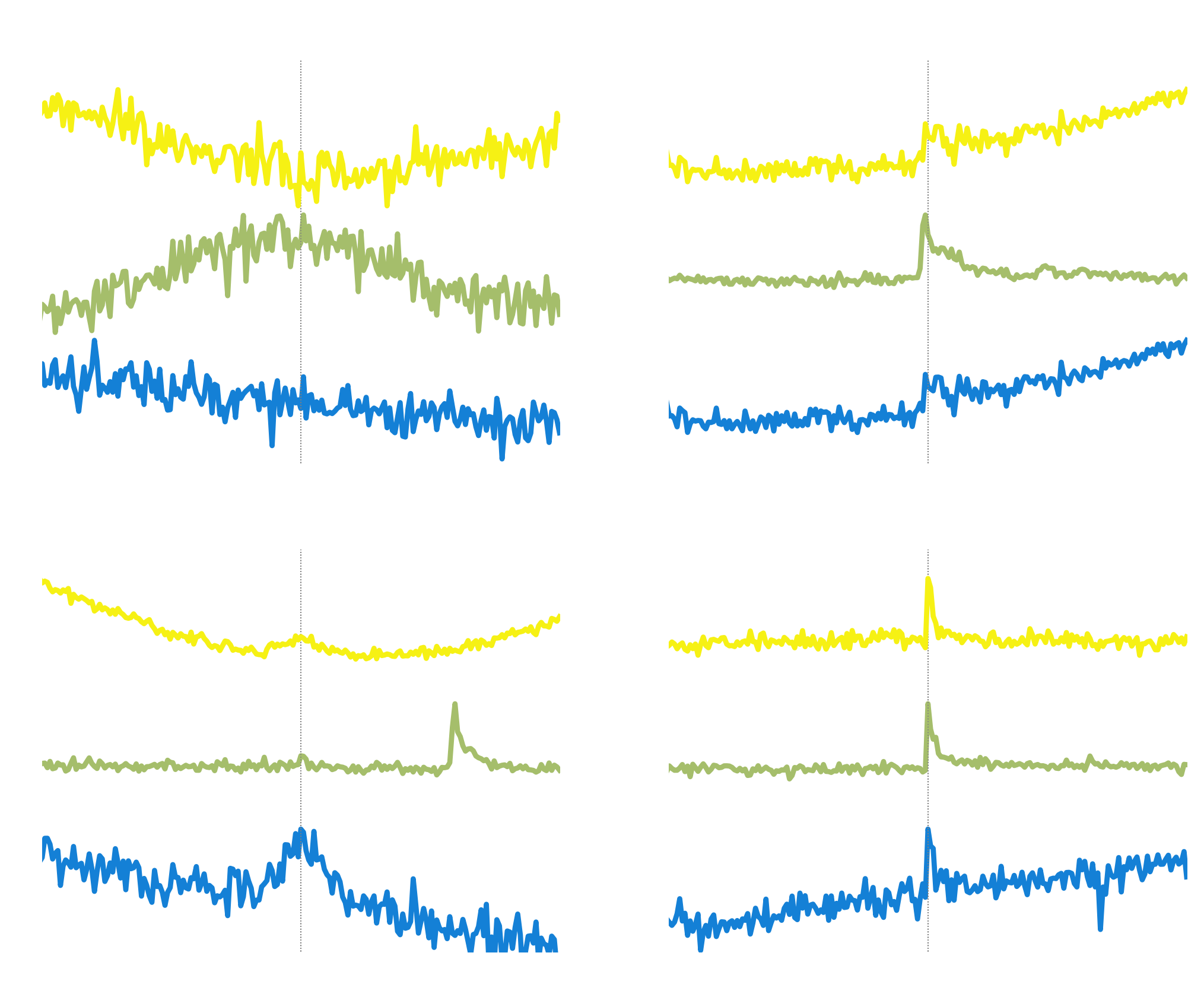
In order to understand the exoplanet population we see today, we must understand the early stages of planet formation and evolution. The star a planet orbit dictates its entire life. It sets the environment the planet resides in. Young stars are known to emit higher X-ray/UV radiation and be more magnetically active. In particular stellar flares, which are caused by the reconnection of magnetic field lines have destructive consequences, such as:

Increased photoevaporation of the inner disk (Benz & Gudel, 2010).
Increased atmospheric erosion, especially for short period planets while they are still forming and contracting (Owen & Wu, 2017).
Long term effects on the chemical compositions of atmospheres (Venot+ 2016).

We used data from the Transiting Exoplanet Survey Satellite (TESS) to detect flares and determine flare rates and evaluate how these values affect the photoevaporoative atmospheric mass loss for close-in planets.

Sample Selection & Machine Learning

Young stars were identified through a literature search. The Gaia kinematics were run through BANYAN-SIGMA to assign each star to a young moving groups, young open clusters, OB associations, or star forming region. In total, we have a sample of 3200 young stars observed at TESS 2-minute cadence in Sectors 1-19.

To identify flares, we trained a convolutional neural network (CNN), stella on the flare catalog from Gunther+2020. The results of the training are shown left. Accuracy is the fraction of predictions the models got correct. The loss tests how far from the true values the network is labeling examples. Thus, a well performing CNN will have accuracy converge to 1 and loss converge to 0, which is what we see in stella.

We can evaluate the confusion matrix for the stella test set. This highlights examples that are:

True Negatives (top left): Non-flares identified as non-flares.
False Positives (top right): Flare-like shapes that could be noise of unlabeled true flares.
False Negatives (bottom left): True flares with shapes that deviate from the typical positive examples.
True Positives (bottom right): Flares identified as flares.

Note the green false positive, which looks like an unlabeled true flares, highlighting the incompleteness of our training set to every flare in the light curves.

With stella we are able to assign a probability that a given cadence is part of a flare. Here is a video demonstration of this: As the CNN moves along the light curve, the two flares light up in yellow, but also in the probability time series, shown in the bottom subplot. By assigning probabilities, which has never been done in other flare detection techniques, we are able to say something truly statistical about flare rates.

What relationships do we find between flare rate and spectral type, age, and spot phase?

Flares are borken down into bins of T_eff and by age (teal = t_age < 50 Myr; yellow = t_age > 50 Myr). Temperature ranges are labeled in each subplot. We note a detection bias towards lower energy flares for cooler stars.

There is a noticeable drop-off in flare rate and energy as the star's temperature increases. M and late K dwarfs (T_eff < 4000 K) experience similar flare rates and energies across the entire age range of our sample. The high-energy flare tail extends out to 10³⁵ergs and is most noticeable for t_age < 50 Myr stars. T_eff > 6200 K corresponds to the Kraft break and thus a change in interal structure, which may be the cause of such a lack of flares.

Here, we plot Gaia color against our measured rotation periods, P_rot. Points are colored by the flare rate of that star. There is a noticeable decrease in flare rate at Gaia B_p> - R_p> = 2, which corresponds to a T_eff = 4000 K. Most stars with color B_p> - R_p> < 2 do not exhibit any flares, while the cooler stars show a variety of flare rates across all rotation periods. There is a clear artificially induced break at P_rot > 12 days, as the result of our rotation period metrics.

We were able to measure rotation periods for 1500 stars in our sample. There is no preference for where flares occur with respect to phase. Here a phase = 0 is the peak of the rotation modulation (i.e. the less spotted hemisphere). Doyle+2018, Doyle+2019, and Doyle+2020 found similar results across smaller samples (30-200) of G and M dwarfs in both K2 and TESS data.

The result presented here is the largest sample of young stars for which such an analysis has been completed.

What do these high flare rates mean for young exoplanets?

Modifying the photoevaporative atmospheric mass loss equation from Owen & Wu (2017), to account for flares, we find that:

When flares are present for the first 200 Myr, 4% more atmospheric mass is lost (green curve).
When flares are present for the first 1000 Myr, 7% more atmospheric mass is lost (yellow curve).

Although these differences when accounting for flares do not seem large, this does suggest that flares need to be accounted for in more detail moving forward.

Flares have been shown to alter atmospheric chemistry. Here, we demonstrate they could partially affect mass-loss rates during formation.