Testing Self-Organized Criticality Across the Main Sequence using Stellar Flares from TESS

Adina Feinstein, Darryl Seligman, Maximilian Gunther, & Fred Adams

arXiv:2109.07011

TL;DR

We use ~10⁶ stellar flares to provide evidence that all stellar coronae may be in self-organized critical states.

What is Self-Organized Criticality?

The theory of self-organized criticality describes a class of dynamical systems which remain at a critical point with no intrinsic length or time scale (Bak, Tang, & Wiesenfeld, 1988). A simple model to see this critical point is a sandpile. Here, the length is the difference in height between neighboring sand grains and it helps to visualize the height difference as steps. When more sand is added to the pile, the pile increases and creates new height differences between neighboring sites (i.e. you make different height steps). When the additional sand grains cause the new height difference to exceed a critical slope, an avalanche event occurs. In this example, the slope of the sandpile, and the fact that post-avalanche the system returns to the same slope, is the critical value.

Self-organized criticality naturally manifests in a variety of physical systems including: forest fires (Turcotte, 1999), landslides (Bak, Chen, & Tang, 1990), neuroscience (Ribeiro et al. 2010), evolution (Bak & Sneppen, 1993), financial markets (Bak, Paczuski, & Shubik, 1997), and Conway's Game of Life (Bak, Chen, & Creutz, 1989) to name a few.

Stellar Flares from TESS

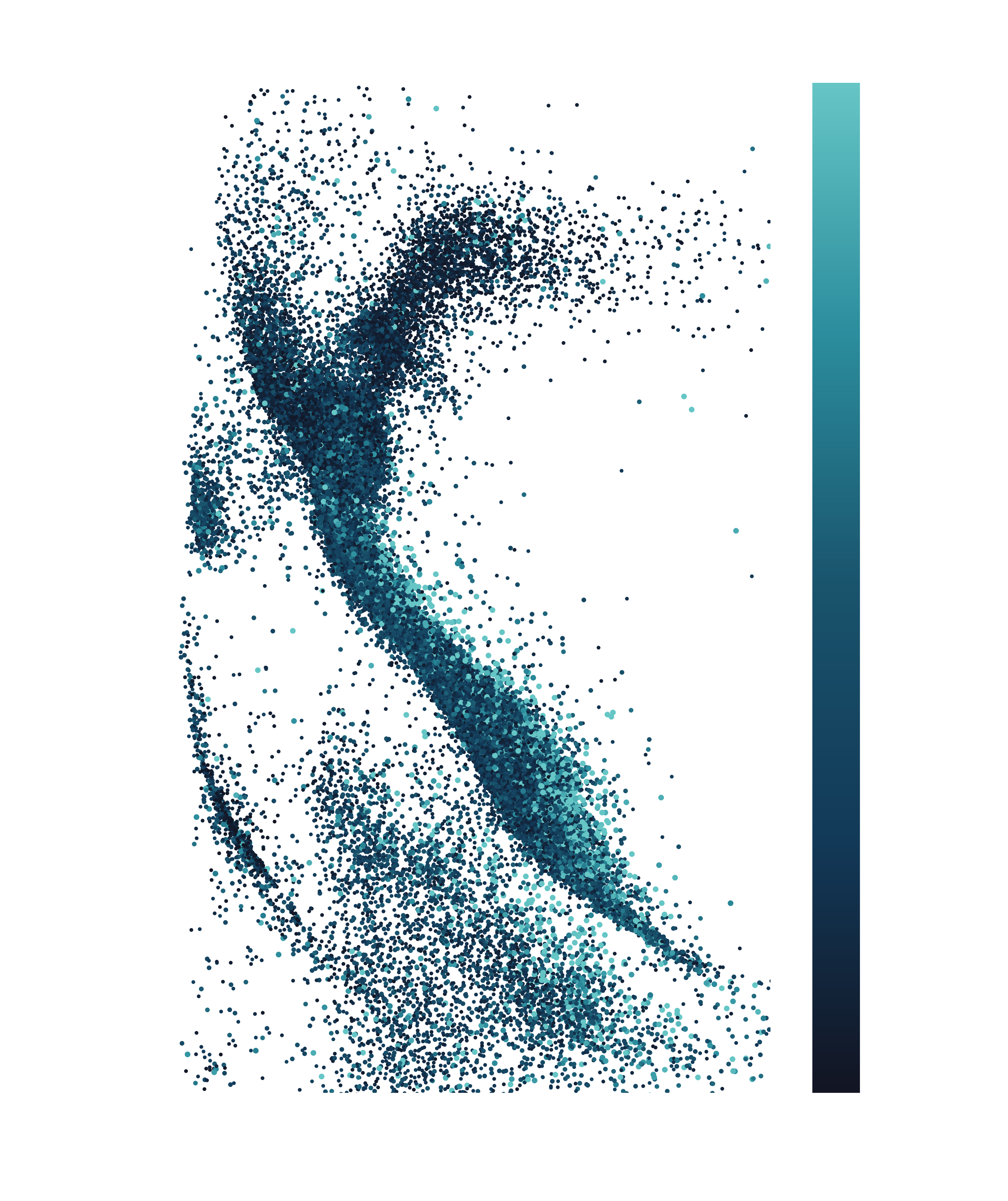
To test if all stellar coronae are in self-organized critical states, we need a large sample of stellar flares across a variety of spectral types. For this, we used all of the stars observed at high cadence by the Transiting Exoplanet Survey Satellite (TESS). This sample has 161,836 stars that are located all across the HR diagram (see left), with the majority of stars falling along the main sequence.

Because we had such a large number of stars, each observed for at least 25 days, we needed a scalable approach to identifying and characterizing flares in the light curves. For this we used the stella convolutional neural networks (CNNs; Feinstein et al. 2020). This technique assigns a probability to each flare (0 = not a flare; 1 = flare), allowing us to statistically validate each event. Due to the small training set of the original CNNs, we additionally apply 4 false positive filters to the data (as prescribed by Gunther et al. in prep):

Signal-to-Noise filter: requires flares to be 3 x the root-mean-square of the data.
Outliers: removes flares with durations < 4 minutes (likely noise).
Eclipsing binaries: removes flares correspond to ingresses/egresses of eclipses, as these can be sharp features that look flare-like.
Variability/Rotation: removes flares that occur at the peak of periodic modulation in the light curve.

This left us with 958,659 flares originating from all sample of stars. We then calculated the flare rate (flares / day) of each star. We weighed each flare by the probability that it is a flare.

Inferring Properties about Stellar Coronae

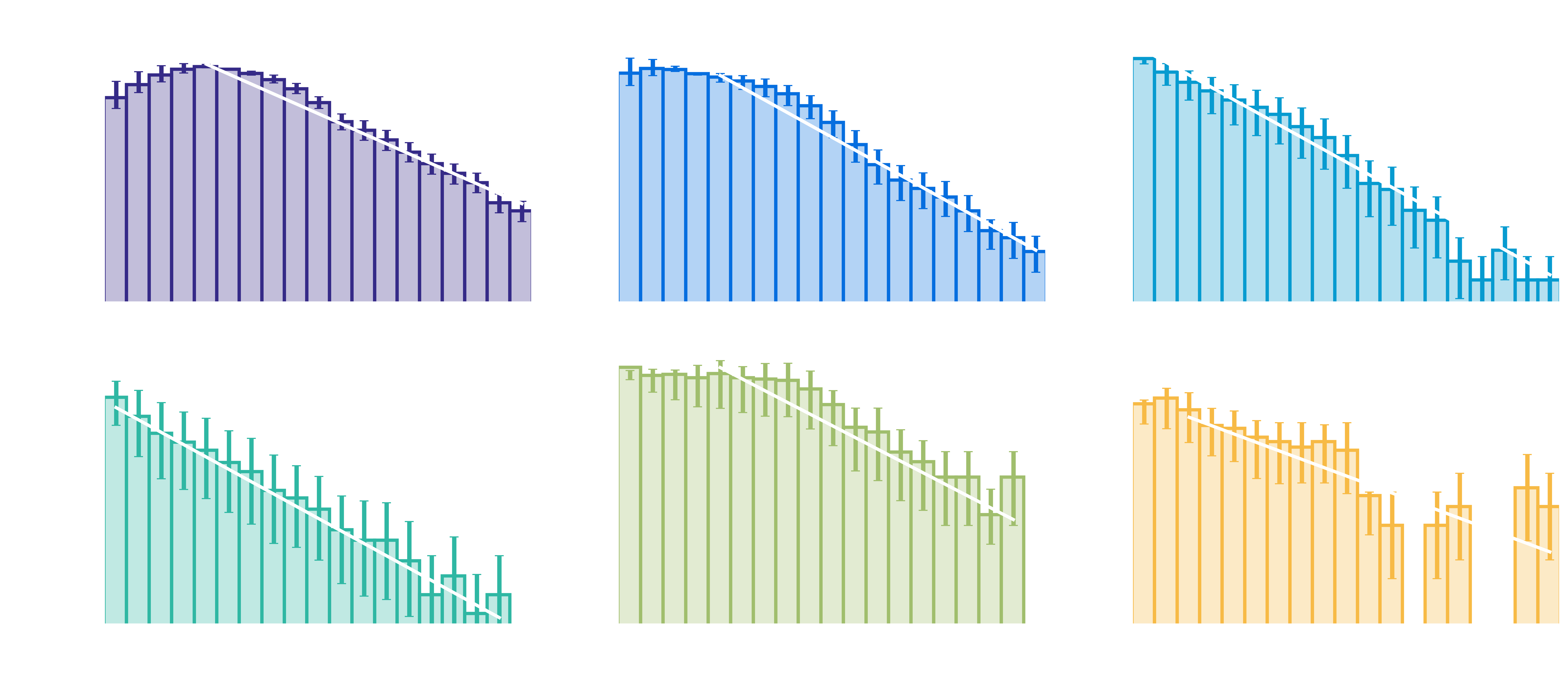
We present our measured flare frequency distributions (FFDs) and slopes above. We broke our sample up into 6 bins: 5 based on stellar mass on the main sequence (purple through green) and 1 bin for stars on the red giant branch (yellow). The histograms represent all flares with probabilities >= 0.9, to provide a high-confident set of flares. We chose to bin the flares by amplitude (%) rather than flare energy to remove additional errors resulting from estimating stellar luminosities. We estimated the upper and lower errors on the FFD as flares with probabilities >= 0.99 and flares >= 0.5.

We find the measured slopes are consistent with models of flaring activity as self-organized critical systems (Lu & Hamilton, 1991) and with that measured for the Sun (de Arcangelis et al. 2006).

compare

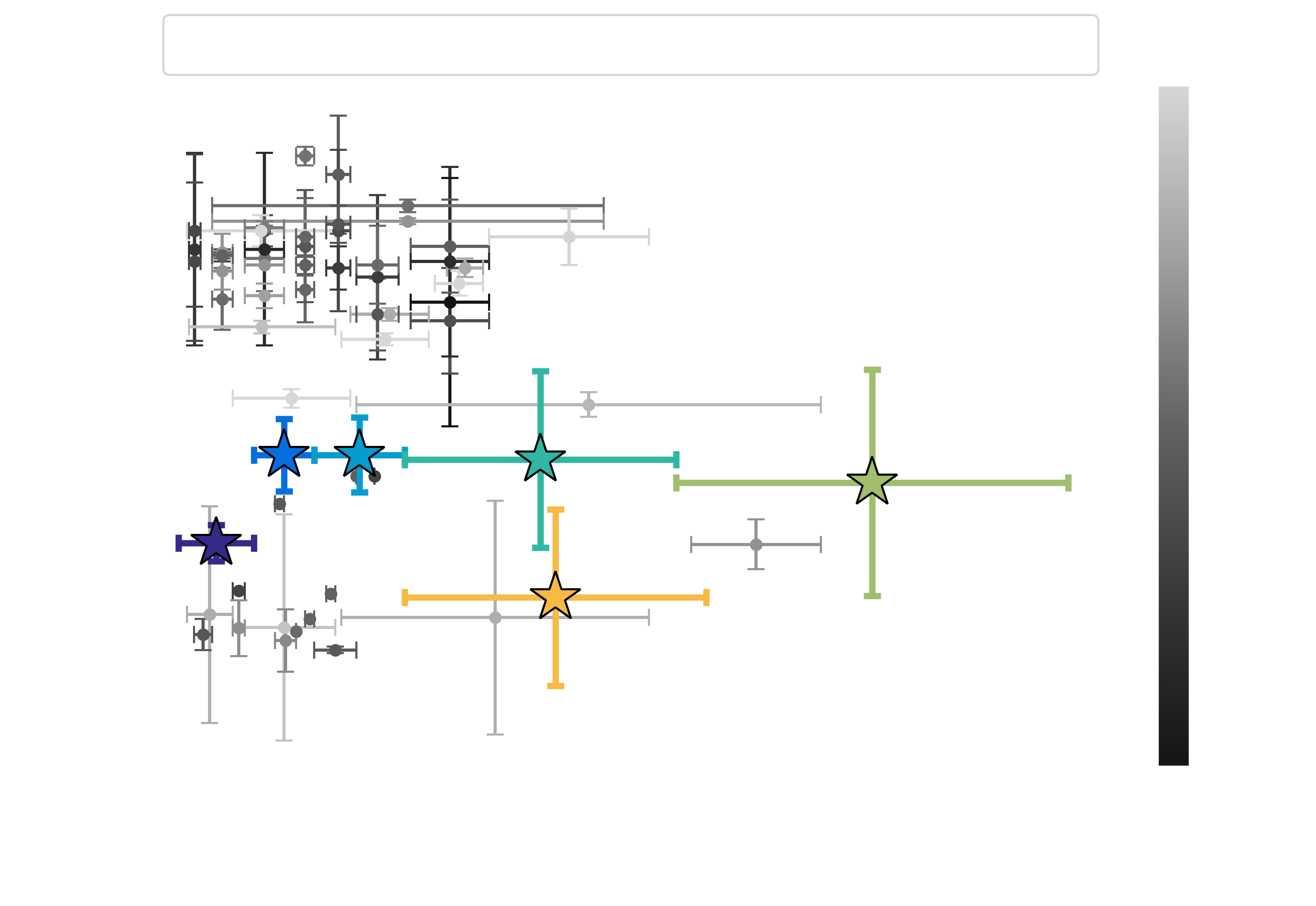
Additionally, we compare our measured FFD slopes to that found in the literature. Previous studies used an order of magnitude fewer flare events and reported steeper slopes than the ones measured here. The variation arises based on sample size/selection and the cadence of the analyzed flares. This variation may also arise from the difference in total observing times.